Hello everyone,
In this thread, I want to propose a new LIP for the roadmap objective “Introduce authenticated data structure”. The purpose of this LIP is to define a generic Merkle Tree structure and a format for proof-of-inclusion that can be used in different parts of the Lisk protocol.
As always, I’m looking forward to your feedback.
Here is the complete LIP draft:
LIP: <LIP number>
Title: Introduce Merkle Trees and Inclusion Proofs
Author: Alessandro Ricottone <alessandro.ricottone@lightcurve.io>
Type: Standards Track
Created: <YYYY-MM-DD>
Updated: <YYYY-MM-DD>
Requires: 00xx "A generic, deterministic and size efficient serialization method"
Abstract
The purpose of this LIP is to define a generic Merkle Tree structure and a format for proof-of-inclusion that can be used in different parts of the Lisk protocol.
Copyright
This LIP is licensed under the Creative Commons Zero 1.0 Universal.
Motivation
A Merkle tree is an authenticated data structure organized as a tree (Fig. 1). The hash of each data block is stored in a node on the base layer, or leaf, and every internal node of the tree, or branch, contains a cryptographic hash that is computed from the hashes of its two child nodes. The top node of the tree, the Merkle root, uniquely identifies the dataset from which the tree was constructed.
Merkle trees allow for an efficient proof-of-inclusion, where a Prover shows to a Verifier that a certain data block is part of the authenticated dataset by sending them a proof with an audit path. The audit path contains the node hashes necessary to recalculate the Merkle root, without requiring the Verifier to store or the Prover to reveal the whole dataset. For a dataset of size N, the audit path contains Log(N) hashes at most, and the proof-of-inclusion is verified by calculating at most Log(N) hashes (here and later Log indicates the base 2 logarithm of the argument). Furthermore, if the Verifier wants to check the presence of multiple data blocks at once, it is possible to obtain some hashes directly from the data blocks and reuse them for multiple simultaneous verifications.
In Bitcoin, the transactions contained in a block are stored in a Merkle tree. This allows for Simplified Payment Verification (SPV), i.e., a lightweight client can verify that a certain transaction is included in a block without having to download the whole block or Bitcoin blockchain.
In Ethereum, the roots of Merkle Patricia trees are included in each block header to authenticate the global state of the blockchain (stateRoot), the transactions within the block (transactionsRoot and receiptsRoot) and the smart contract data (storageRoot for each Ethereum account).
The inclusion of Merkle trees can be beneficial in several parts of the Lisk protocol:
- Storing the root of a Merkle tree for the transactions in the
payloadHashin the block header would allow users to verify efficiently that a transaction has been included in the block. At the moment thepayloadHashcontains the hash of the serialized transactions, and to verify the presence of a single transaction users have to download the whole block. After the proposed change to limit the block size to 15kb, a full block will contain approximately 120 transactions at most. In this case, performing a proof-of-inclusion will require to query 7 hashes, and the size of the corresponding proof would be 232 bytes (see “Proof serialization” section below). Thus, the amount of data to be queried to verify the presence of a single transaction in a full block is reduced by ~98%; - Merkle trees as an authenticated data structure can be helpful to create a snapshot of the account states as well as the transaction and block history, for example for the “Introduce decentralized re-genesis” roadmap objective.
Rationale
This LIP defines the general specifications to build a Merkle tree from a dataset, calculate the Merkle root and perform a proof-of-inclusion in the Lisk protocol. We require the following features:
- Cryptographically secure: the dataset can not be altered without changing the Merkle root;
- Proof-of-inclusion: presence of data blocks in the dataset or in the tree can be verified without querying the whole tree;
- Efficient append: new data blocks can be appended to the dataset, and the tree is updated with at most Log(N) operations for a dataset of size N.
We consider two possible implementations for a Merkle tree: regular Merkle trees (RMT) and sparse Merkle trees (SMT).
Regular Merkle Trees
In a RMT, data blocks are inserted in the tree in the order in which they appear in the dataset. Hence, the order can not be altered to reproduce the same Merkle root consistently. This also implies that in a RMT it is not possible to insert a new leaf in an arbitrary position efficiently, as this changes the position in the tree of many other leaf nodes, so that the number of branch nodes to be updated is proportional to the size of the tree N. On the other hand, RMTs are suitable for append-only dataset, as appending a new elements to the dataset updates a number of branch nodes proportional to Log(N) only.
RMT accepting input data blocks with arbitrary length are susceptible to second pre-image attacks. In a second pre-image attack, the goal of the attacker is to find a second input x′ that hashes to the same value of another given input x, i.e. find x’ ≠ x such that hash(x) = hash(x’). In Merkle trees, this corresponds to having two different input datasets x and x’ with the same Merkle root. This is trivial in an RMT: choose x = [D1, D2, D3, D4] and x’ = [D1, D2, hash(D3) | hash(D4)], where | indicates input concatenation. To solve this problem we use a different hashing function for leaf and branch nodes [1].
RMTs are in general easier to implement because of their limited storage requirements. Furthermore, the dataset can be sorted in such a way that most queries would ask for a proof-of-inclusion for data blocks stored consecutively, allowing then for smaller audit paths. For example this is the case for the Merkle tree build out of blocks headers where blocks are stored according to their height, and a typical query could ask to verify the presence of consecutive blocks in the blockchain.
Sparse Merkle Trees
In a SMT, all possible leaf nodes are initialized to the empty value. Every leaf occupies a fixed position, indexed by its key. In a SMT, the order of insertion of the data blocks is not relevant, as all leaf nodes are indexed by their respective keys.
In a SMT it is possible to obtain a proof-of-absence for a certain key by simply showing that the empty value is stored in the corresponding leaf with a proof-of-inclusion. SMTs are easy to update: once a leaf node with a certain key is updated, one has to update only Log(N) branch nodes up the tree. For 256 bits-long keys, there are 2256 possible leaf nodes, and the height of the tree is 256. Hence, each update changes the value of 256 nodes.
SMT are too large to be stored explicitly and require further optimization to reduce their size. For example, one could decide to place a leaf node at the highest subtree with only 1 non-null entry and trim out all empty nodes below it. This is the approach taken by the Aergo State trie.
We choose to implement RMTs and reserve the possibility to implement SMTs in different parts of the Lisk protocols in the future.
Proof-of-Inclusion Protocol
In this section, we clarify the steps necessary for a proof-of-inclusion and introduce some useful terminology. The elements constituting a proof-of-inclusion are:
-
merkleRoot: The Merkle root of the tree built from the datasetdata; -
queryData: A set of data blocks to be verified. This set is not necessarily a subset ofdata, as it may contain hash values of branch nodes, which we allow to be verified. -
proof: The proof itself, consisting of 3 parts:dataLength,idxsandpath:-
dataLength: The total number of data blocks in the dataset (the length ofdata); -
idxs: A set of indices corresponding to the position in the tree of the data inqueryData; -
path: The audit path, an array ofbytesnecessary to compute the Merkle root starting fromqueryData.
-
The procedure for a proof-of-inclusion is as follows:
-
Verifier:
The Verifier knowsmerkleRootand sends the Prover a set of data blocksqueryDatafor which they wish to obtain a proof-of-inclusion; -
Prover:
- The Prover finds the elements of
queryDatain the Merkle tree and generates the set of corresponding indicesidxs; - The Prover generates
pathand transmits the completeproofto the Verifier;proofcontainsdataLength,idxsandpath;
- The Prover finds the elements of
-
Verifier:
The Verifier usesproofto recalculate the Merkle root using elements fromqueryDataand checks that it equalsmerkleRoot.
In Fig. 1 we sketch a simple proof-of-inclusion for data block data1. The Verifier asks the Prover for a proof for queryData=[data1]. The Prover sends back proof with dataLength=5, idxs=[0001]and path=[h0, h6, h4].
Specification
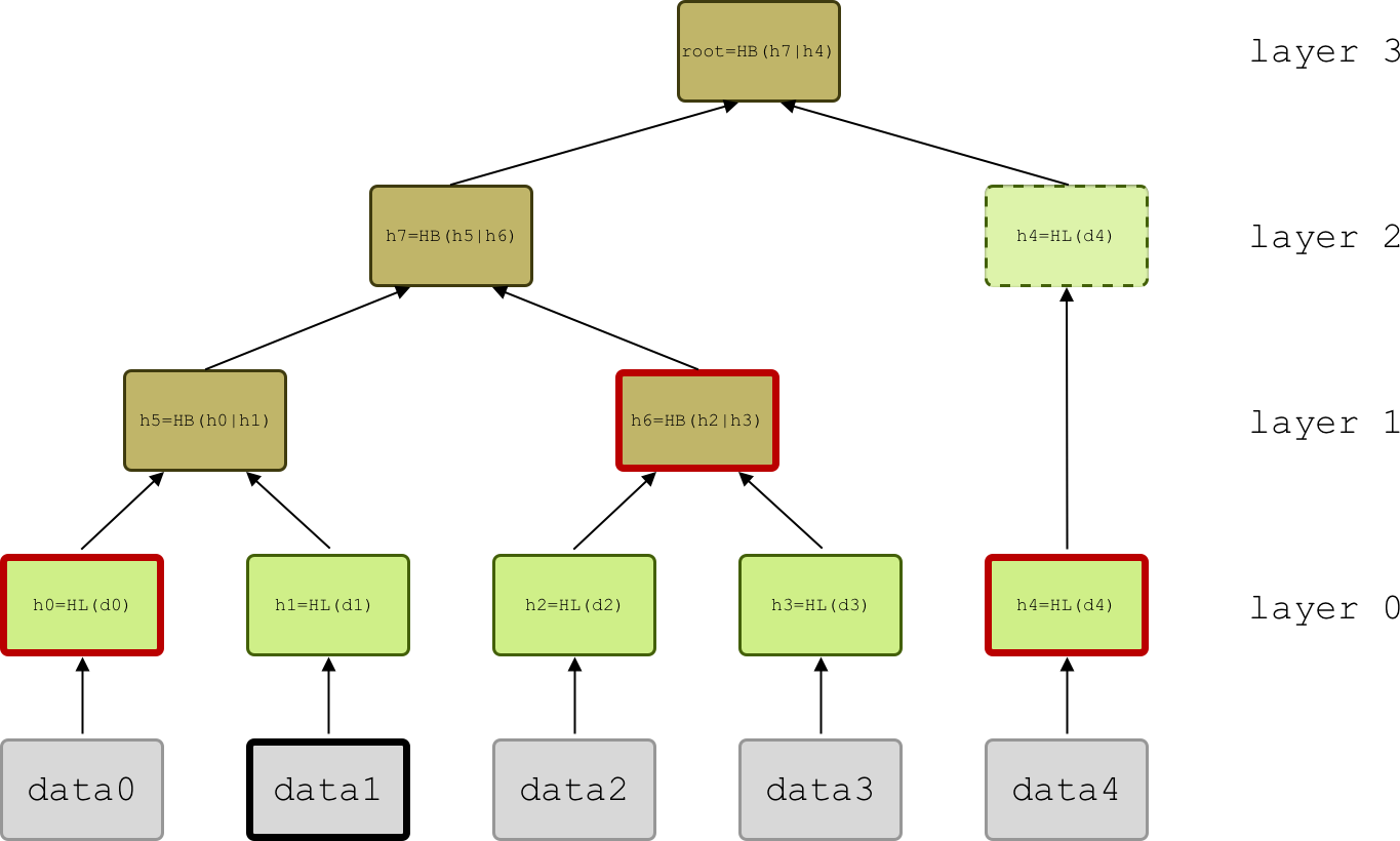
Figure 1: A Merkle tree built from the dataset
[data0, ...data4]. Here N=5. The leaf hash HL=LEAFHASH of the data blocks (grey rectangles) is inserted as leaf node (green rectangles). Branch nodes (brown rectangles) contain the branch hash HB=BRANCHHASH of two children nodes below them. Unpaired nodes are just passed up the tree until a pairing node is found. The path for data1 (red-bordered rectangles) includes h0, h6 and h4 in this order. The layers of the tree, starting from the bottom, have 5, 2, 1 and 1 nodes.
In this section we define the general construction rules of a Merkle tree. Furthermore, we specify how the Merkle root of a dataset is calculated and how the proof construction and verification work. The protocol to efficiently append a new element to the tree is specified in Appendix B.
We assume data blocks forming the dataset are bytes of arbitrary length, and the hash values stored in the tree and the Merkle root are bytes of length 32. We define the leaf- and branch-nodes hash function by prepending a different constant flag to the data before hashing [1, Section 2.1. “Merkle Hash Trees“]:
LEAFHASH(msg) = HASH(LEAFPREFIX | msg);BRANCHHASH(msg) = HASH(BRANCHPREFIX | msg),
where | indicates bytes concatenation and LEAFPREFIX and BRANCHPREFIX are two constants set to:
LEAFPREFIX = 0x00;BRANCHPREFIX = 0x01.
Here the function HASH returns the SHA-256 hash of the input. Data blocks from the dataset are hashed and inserted in the tree as leaf nodes. Then nodes are hashed together recursively in pairs until the final Merkle root is reached. If N is not a power of two, some layers will have an odd number of nodes, resulting in some nodes being unpaired during the construction of the tree. In this case we just pass the node to the level above without hashing it (Fig. 1 where N=5).
Merkle Root
For an input dataset of arbitrary length of the form:
-
data: An (ordered) array ofbytesof arbitrary length,
we define a unique bytes value of length 32, the Merkle root merkleRoot.
The Merkle root is calculated recursively by splitting the input data into two arrays, one containing the first k data blocks and one for the rest, where k is the largest power of 2 smaller than N, until the leaf nodes are reached and their LEAFHASH is returned [1]. Notice that the order of the input array matters to reproduce the same Merkle root.
merkleRoot(data) {
  dataLength = data.length
  if (dataLength == 0) return EMPTYHASH
  if(dataLength == 1) return LEAFHASH(data[0])
  k = largestPowerOfTwoSmallerThan(dataLength)
  #split the data array into 2 subtrees. leftTree from index 0 to index k (not included), rightTree for the rest
  leftTree = data[0:k]
  rightTree = data[k:dataLength]
  return BRANCHHASH(merkleRoot(leftTree) | merkleRoot(rightTree))
}
The Merkle root of an empty dataset is equal to the hash of an empty string: EMPTYHASH=SHA256().
Proof-of-Inclusion
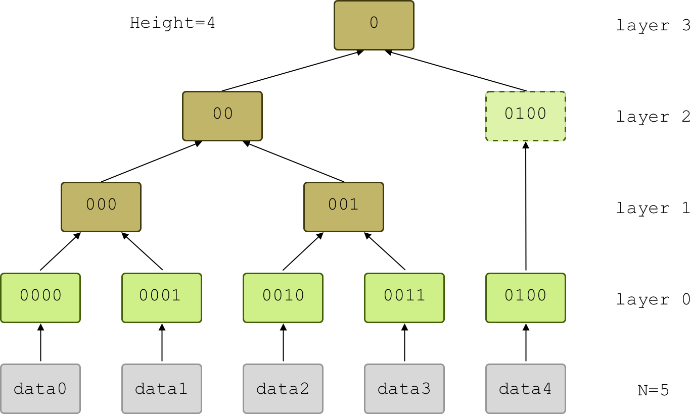
Figure 2: An indexed Merkle tree. The binary index uniquely identifies the position of each node in the tree: the length of the index, together with the tree height, specifies the layer the node belongs to, while the index specifies the position within the layer.
For an input dataset of arbitrary length of the form:
-
queryData: an array ofbytesof arbitrary length,
we define an array proof containing 3 parts:
-
dataLength: The total length of the datasetdata; -
idxs:An array indicating the position in the datasetdataof the elementsqueryDatato be verified; -
path:An array ofbytes, containing the node values necessary to recompute the Merkle root starting fromqueryData.
Proof Construction
The Prover searches for the position in the tree of each data block in queryData, and generates the corresponding array idxs assigning an index to the data block according to the following rules:
- If the data block is not part of the tree, it is assigned a special index (see “Proof serialization” section), and the data block is not taken into consideration when constructing the rest of the proof;
- The index of a data block present in the tree equals its position in the layer converted to binary, with a fixed length equal to the tree height minus the layer number, with
0s prepended as necessary (see Fig. 2). Notice that in this representation each index starts with a0, and the layer the node belongs to can be inferred from the length of the index anddataLength.
Notice that the elements of idxs are placed in the same order as the corresponding data in queryData and not sorted. The Prover generates the path by adding the necessary hashes in a bottom-up/left-to-right order. For the example in Fig.1, starting from the base layer and the leftmost node, the hash values added to the path are h0, h6 and h4. This order reflects the order in which the path is consumed by the Verifier during the verification.
Proof Serialization
The proof is serialized according to the specifications defined in LIP 00xx “A generic, deterministic and size efficient serialization method” using the following JSON schema:
proof = {
    "type": "object",
    "properties": {
        "dataLength": {
            "dataType": "uint32",
            "fieldNumber": 1
        },
        "idxs": {
            "type": "array",
            "items": {
                "dataType": "uint32"
            },
            "fieldNumber": 2
        },
        "path": {
            "type": "array",
            "items": {
                "dataType": "bytes"
            },
            "fieldNumber": 3
        },
    },
    "required": [
        "dataLength",
        "idxs",
        "path"
    ],
}
In particular:
-
dataLengthis encoded as auint32; - Each index in
idxsis prepended a1and is encoded as auint32. The extra1is added as a delimiter to set the correct index length. At the moment of decoding, each index is converted from unsigned integer to binary, the first bit (which equals1) is dropped and only the following bits are kept. Furthermore, we use the special index0to flag any element which is not part of the dataset, and as such can be discarded during the verification. Notice that this does not constitute a proof-of-absence for that element; - The elements of
pathare encoded as an array ofbytesof length 32.
The hex-encoded proof for the example in Fig. 1 is proof=0x0805|0x120111|0x1a20|h0|0x1a20|h6|0x1a20|h4, with a length L=107 bytes.
Verification
The Verifier obtains dataLength from the proof, and calculates the structure of the tree from dataLength. In particular, they know how many nodes are present in each layer with the following simple rule:
- There are a total number of layers equal to
Height=ceiling(Log(dataLength))+1; - The base layer contains a number of nodes equal to
dataLength; - Each other layer contains half the number of nodes of the layer below. If this is an odd number, we round either down and up, alternating every time it is necessary and starting by rounding down.
For example, to dataLength=13 corresponds Height=5 and #nodesPerLayer=[13, 6, 3, 2, 1].
With the structure of the tree and idxs, the Verifier is able to identify the position in the tree of each element of queryData and to drop all elements that are not part of the tree using the special flag. They consume the path in the same order in which it was constructed to calculate the Merkle root. Finally, they check that the resulting Merkle root equals merkleRoot to complete the verification.
Backwards Compatibility
This proposal does not introduce any forks in the network, as it only defines the specification to build a Merkle tree in the Lisk protocol. Future protocol changes involving the introduction of Merkle trees (such as LIP 00xx “Replace payloadHash with Merkle tree root in block header” or the “Introduce decentralized re-genesis” roadmap objective) will require this proposal.
Appendix A: Proof-of-Inclusion Implementation
We describe two functions to perform a proof-of-inclusion:
generateProof(queryData): return proof;verify(queryData, proof, merkleRoot): return check;
We split generateProof into 3 different subroutines, one for each part of the proof (see section “Proof-of-inclusion”):
generateProof(queryData) {

  1. getdataLength(){
    return dataset.length
  }

  2. getIndices(queryData){
    for elem in queryData:
      find node with node.hash == elem or node.hash == LEAFHASH(elem)
      if node not in tree:
        idx = constant value to flag missing nodes
      else:
        idx = binary(node.index), with length = height - node.layer
      push idx to idxs
    return idxs
  }

  3. getPath(idxs) {
    for idx in idxs:
      if idx == missing node flag:
        remove idx from idxs and continue
      find pair
      #Notice that pair node could come from a lower layer
      if node is unpaired:
        pass
      else if pair.index in idxs:
        remove pair.index from idxs
      else:
        push pair to path
      remove idx from idxs
      #parent index is idx without last bit
      parentIndex = idx >> 1
      push parentIndex to idxs
    return path
  }

  dataLength = getdataLength()
  idxs = getIndices(queryData)
  path = getPath(idxs)
  return proof = [dataLength, idxs, path]
}
verify works similarly to generateProof, but stores the known nodes in a dictionary and gets missing nodes from path instead of adding them to it.
verify(queryData, proof, merkleRoot) {
  [dataLength, idxs, path] = proof
  #tree is a dictionary where we store the known values.
  #the key is the index,
  #the value is the corresponding node in the tree (from queryData)
  tree  = {idx: node for idx in idxs}
  for idx in idxs:
    if idx == missing node flag:
      discard idx and continue
    node = tree[idx]
    #the index of the pair is found from dataLength
    #which defines the structure of the tree
    find pairIndex
    #notice that pair node could come from a lower layer
    #parent index is idx without last bit
    parentIndex = idx >> 1
    if node is unpaired:
      pass
    else:
      if pairIndex in tree:
        pair = tree[pairIndex]
      else:
        pair = path[0]
  path = path[1:]
      if node.side == left:
        tree[parentIndex] = parentNode
                            with parentNode.hash = BRANCHHASH(node.hash | pair.hash)
      else:
        tree[parentIndex] = parentNode
                            with parentNode.hash = BRANCHHASH(pair.hash | node.hash)
    remove idx from idxs
    push parentIndex to idxs
  root = tree["0"]
  return root.hash == merkleRoot
}
Appendix B: Append-Path Implementation
Figure 4: Some examples of append paths for Merkle trees of size 2 to 6. On the left of each tree, the binary representation of their respective size is indicated, top to bottom. Whenever a 1 is present, a node in the layer is part of the append path, which therefore contains at most a number of elements equal to Log(N).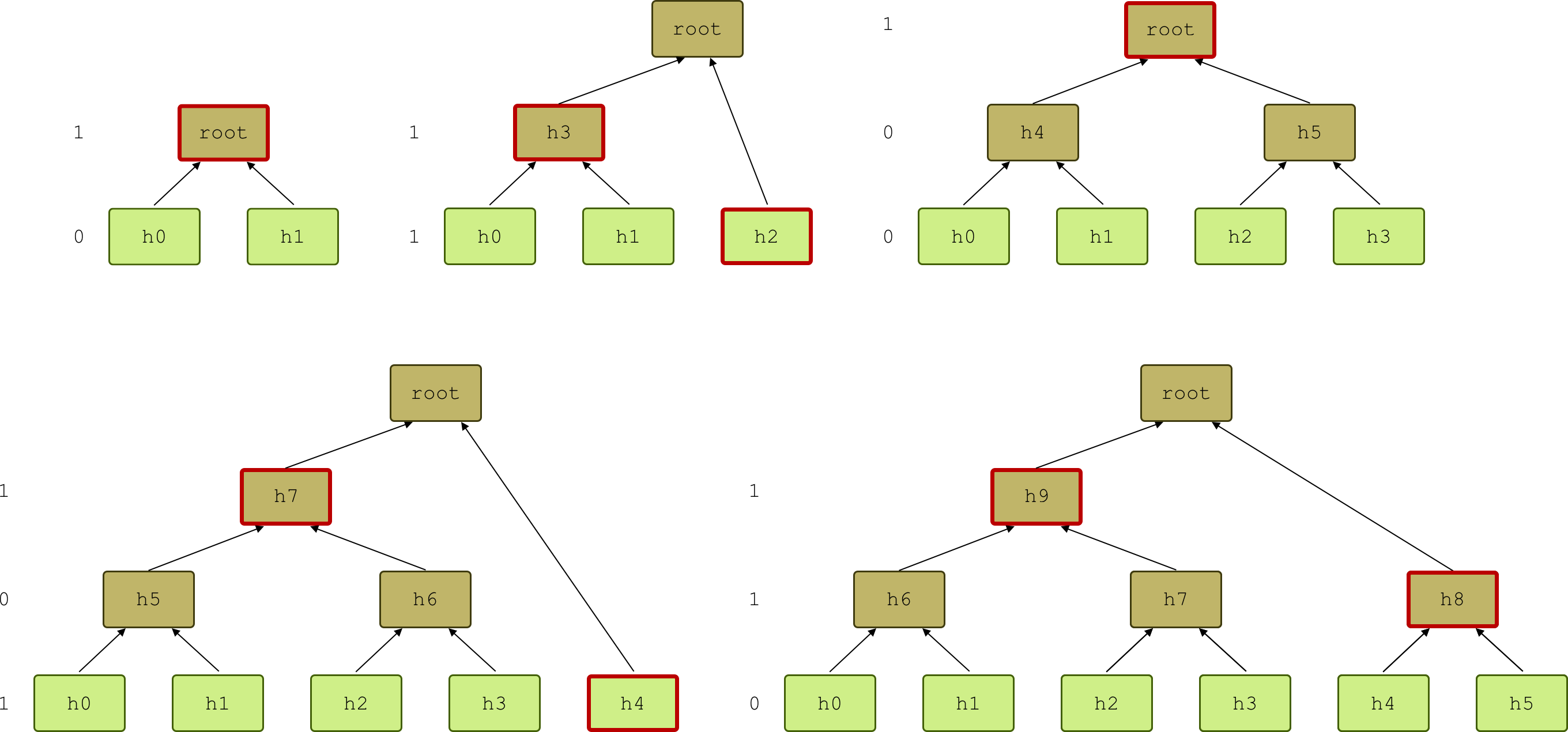
Adding new data blocks to the tree updates the value of at most Log(N) branch nodes. We define the append path to be an array of bytes containing the branch-node values necessary to compute the updated tree (Fig. 4). Adding new data blocks updates the append path as well. Each layer with an odd number of nodes contains a node which is part of the append path. Therefore, the append path contains at most Log(N) elements, and updating the tree requires to calculate at most Log(N) hashes.
To append a new element we need to do the following:
- Add the leaf hash of the element to the base layer;
- Update the affected branch nodes in the tree;
- Update the append path.
In some circumstances, one can be interested in checking that a new data block has been appended correctly to the tree. This can be done without storing the whole tree by recomputing the new Merkle root. In this case it is sufficient to store and update the dataset length, the append path and the Merkle root.
In the following pseudocode, the function append takes as input the new data block newElement and updates the Merkle tree. The strategy is to use the binary representation of dataLength: each digit di ∈ {0, 1} labels a layer of the tree according to the power of 2 it represents, starting with the rightmost digit d0 for the base layer (Fig. 4). Possibly the root has no digit assigned to it (in this case we can assign it a 0).
append(newElement) {

1. hash = LEAFHASH(newElement)
   push hash to base layer
2. k=0
   binaryLength = binary(dataLength)
   #Loop on binaryLength from the right, corresponding to starting from the bottom layer of the tree (see Fig. 4). d = {0, 1} is the current digit in the loop.
   for d in reversed(binaryLength):
     if d == 1: hash = BRANCHHASH(appendPath[k] | hash)
       if k == 0: push hash to above layer, creating a new node
       else: set the value of the last element of the above layer to hash
       k++
3. for d in reversed(binaryLength):
     if d == 0: break loop, set breakIdx = index of d in reversed(binaryLength)
     #if no 0s in binaryLength, breakIdx = binaryLength.length
   #Split appendPath into bottomPath = appendPath[:breakIdx] (bottom layers) and topPath = appendPath[breakIdx:] (upper layers).
   bottomPath = appendPath[:breakIdx]
   topPath = appendPath[breakIdx:]
   #Hash the new element recursively with the hashes in bottomPath
   for h in bottomPath:
     hash = BRANCHHASH(h | hash)
   #The new append path contains the final hash concatenated with topPath
   newAppendPath = [hash] + topPath
}
Appendix C: Merkle Aggregation
Merkle trees can support efficient and verifiable queries of specific content through Merkle aggregation [2]. In a Merkle aggregation, extra information is stored on each node of the Merkle tree as a flag. When a new leaf is appended to the tree, its flag is included in the hash, for example by prepending it to the leaf node value, and is stored together with the resulting hash in a tuple leafNodeValue=(flag, HASH(flag | LEAFPREFIX | message) ). A parent node combines the flags from its children nodes and stores them branchNodeValue=(flag, HASH(flags | BRANCHPREFIX | childrenHashes) ).
The Verifier can then query the Merkle tree for all those elements containing a given flag. The Prover constructs a pruned Merkle tree, where each subtree not containing any flagged node is removed and only the highest node in the pruned subtree is appended to the result. The Verifier can check that each pruning has been done correctly by asking for an inclusion proof for a leaf node in that pruned subtree. They can then verify that the leaf node did not contain the flag. Therefore, the Verifier receives a list of flagged events with a proof that no event is missing from the list (no false positives).
If we want to allow for F different flags, each node will store an F-bits array. Each flag is set by setting the corresponding bit to 1, and branch nodes apply bitwise or on the children-nodes flags.
Appendix D: Example of Proof-of-Inclusion Protocol for Transaction IDs
As an example, the following procedure can be used to verify the presence of a set of transactions in a block.
-
Client:
- Choose a set of transaction IDs
queryIDsand a block IDblockID. We assume the client already knows the Merkle rootmerkleRoot. - Ask the server (for example a full node) for the
proofnecessary to verify the transactions corresponding toqueryIDs, for example with a get request passing(queryIDs, blockID)as parameters.
- Choose a set of transaction IDs
-
Server:
3. Get block fromblockID. IfblockIDdoes not give a valid block, return an emptyproof.
4. Get the list of transactions from the block payload and their IDstxIDs.
5. Get the indicesidxsof the requestedqueryIDsintxIDs. If a transaction is not intxIDsset its index to a flag indicating that it is not part of the block.
6. Generate thepath.
7. Transmitproof=[blockTxs.length, idxs, path]. -
Client:
8. ReorderqueryIDsbased on the order in which the indices inidxsare given. If a transaction was not part of the block, drop it fromqueryIDs.
9. Verify the presence of the transactions callingverify(queryIDs, proof, merkleRoot).
References
[1] Laurie, B., Langley, A. and Kasper, E., 2014. Certificate Transparency. ACM Queue, 12 (8), pp.10-19.
https://tools.ietf.org/html/rfc6962
[2] Crosby, S.A. and Wallach, D.S., 2009, August. Efficient Data Structures For Tamper-Evident Logging. In USENIX Security Symposium (pp. 317-334).
http://static.usenix.org/event/sec09/tech/full_papers/crosby.pdf